
Stablility of Fixed Point of a Dynamical System
Published:
Stability theory is used to address the stability of solutions of differential equations. A dynamical system can be represented by a differential equation. The stability of the trajectories of this system under perturbations of its initial conditions can also be addressed using the stability theory.
Fixed Point
Consider a dynamical system given by the following ordinary differential equation (ODE):
\[\dot x = f(x)\]A fixed point of this system is given by:
\[\dot x = 0\]Therefore, \(f(x) = 0\) or roots of the function \(f(x)\) form the fixed points of the dynamical system.
Stable and Unstable Fixed Points
In layman’s terms, you can say the following about stable and unstable fixed points.
Stable Fixed Point: Put a system to an initial value that is “close” to its fixed point. The trajectory of the solution of the differential equation \(\dot x = f(x)\) will stay close to this fixed point.
Unstable Fixed Point: Again, start the system with initial value “close” to its fixed point. If the fixed point is unstable, there exists a solution that starts at this initial value but the trajectory of the solution will move away from this fixed point.
In other words, one can also think of a stable fixed point as the attractor and unstable fixed point as the repeller. A particle governed by \(\dot x = f(x)\), a stable fixed point will force this particle to move towards itself. On the other hand, an unstable fixed point will force a particle away from itself.
Mathematical Intuition:
For a dynamical system, \(\dot x = f(x)\), a fixed point is \(f(x) = 0\).
If \(f^{\prime}(x) \gt 0\), we have magnitude of \(f(x)\) increasing at x. This can be represented as \(f(x - \delta) \lt 0 \lt f(x + \delta)\) for a sufficiently small value of \(\delta \gt 0\).
Thus, if we start from \(x+\delta\) which is “close” \(x\), the ODE from equation (1) will keep on increasing the value of $x$. And it we start from \(x-\delta\) which is “close” \(x\), equation (1) will move the particle way from \(x\) by decreasing the value of \(x\).
Therefore, if \(f^{\prime} (x) \gt 0\), we have an unstable fixed point and vice versa.
Note: The condition of \(f^{\prime} (x) \lt 0\) or \(f^{\prime} (x) \gt 0\) are sufficient conditions to guarantee fixed point stability or unstability respectively. These are not the necessary conditions, i.e., it is possible to have stable and unstable fixed points where \(f^{\prime} (x) = 0\).
Intuitive Example:
For the differential equation \(x^{\prime} = sin(x)\):
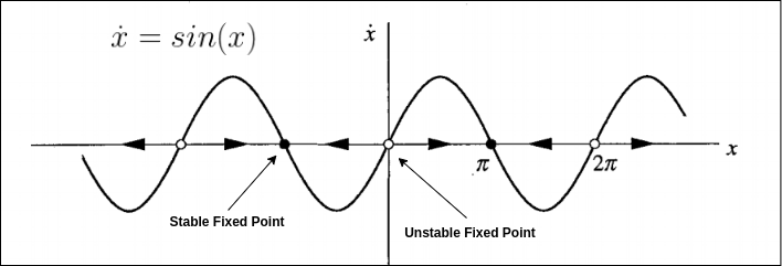
Using linear stability analysis, fixed points occurs when \(f(x)=sin(x)=0\) or \(x=kπ\) where \(k\) is integer.
\(f^{\prime}(x)=cos(kπ)=1\) if \(k\) is even. and \(f^{\prime}(x)=cos(kπ)=−1\) if \(k\) is odd.
Therefore, \(x\) is unstable when \(k\) is even, and stable if \(k\) is odd.
High Dimensional Dynamical Systems
This post discussed the definition of a fixed point of a dynamical system. A simple one-dimensional dynamical system is used as an illustration to explain the concept. A more detailed discussion on general nonlinear, continuous-time, multi-dimensional dynamical systems and their fixed points is provided in my next post.
Leave a Comment