Quadcopter Dynamics and Control

These are my notes on quadcopter dynamics and control from my grad school days.

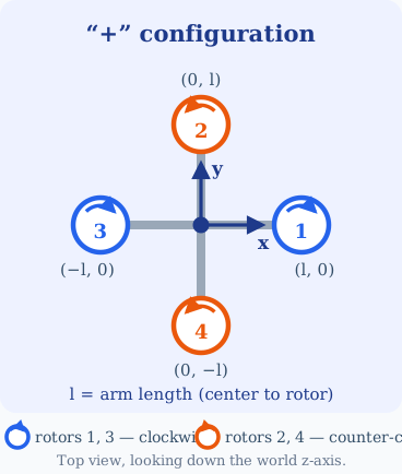
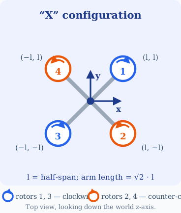
A quadcopter has six degrees of freedom and four actuators, so it is underactuated. Thrust acts along a single body axis. Two rotor layouts are common. The + layout puts one rotor on each body axis, so the nose looks straight past rotor 1. The X layout puts one rotor on each diagonal, so the nose points into the gap between rotors 1 and 2. The key differences in both layouts is of the geometry, the roll and pitch torques the four rotors can produce, and the mixer that turns four scalar demands back into four rotor thrusts. The rigid-body model is the same for both airframes, and so is the cascaded position-and-attitude controller built on top of it.

Most papers state the equations of motion and then produce a finished mixer matrix a line or two later, for one layout only. The steps in between are left to the reader: where the small-angle approximation gets used, why yaw is treated differently from roll and pitch, how four rotor thrusts come out of four scalar demands, and what has to change when the same airframe is rotated by 45 degrees.

I hope someone finds these notes useful.

Conventions used here

Every sign below depends on the four choices listed here, and textbooks differ on all four. Mixing conventions between two sources produces equations that look correct term by term while carrying a sign error in one axis. That error usually survives simulation and shows up on hardware as a roll or pitch loop that diverges. Read this section before comparing anything below against another reference.

1. The world frame is z-up (an ENU-style frame). Gravity therefore acts along $-z_{world}$.
2. The body frame has $x_{b}$ forward, $y_{b}$ left, $z_{b}$ up. Total rotor thrust acts along $+z_{b}$.
3. Attitude uses intrinsic z-y-x Euler angles: yaw $\psi$ about the current $z$, then pitch $\theta$ about the new $y$, then roll $\phi$ about the new $x$.
4. Angular velocity $\boldsymbol\omega = (p, q, r)^{T}$ is expressed in the body frame; the inertia tensor is written in the body frame too, which is what makes it constant.

If you work in a NED frame (z-down, thrust along \(-z_{b}\)), a number of the signs below flip.

Notation

Symbol	Description
\(m\)	mass of the quadrotor
\(g\)	acceleration due to gravity
\(l\)	moment arm about the body \(x\) and \(y\) axes; step 1 gives its geometric meaning, which differs between the two layouts
\(L\)	distance from the center of mass to a rotor hub, used in step 8 to compare the layouts at equal frame size
\(k_f\)	rotor thrust (force) coefficient
\(k_m\)	rotor drag (moment) coefficient
\(\omega_i\)	angular speed of rotor \(i\)
\(F_i, M_i\)	thrust and reaction moment produced by rotor \(i\)
\(i_{xx}, i_{yy}, i_{zz}\)	principal mass moments of inertia about the body \(x, y, z\) axes
\(\phi, \theta, \psi\)	roll, pitch, yaw
\(p, q, r\)	body angular rates about \(x_b, y_b, z_b\)
\(\mathbf{x} = (x,y,z)^T\)	position of the center of mass in the world frame

The state is 12-dimensional, \((\mathbf{x}, \dot{\mathbf{x}}, \phi, \theta, \psi, p, q, r)\), and the input is 4-dimensional, \((\omega_1, \omega_2, \omega_3, \omega_4)\).

The derivation

NOTE: For the following derivation, when a step holds for both airframes the row spans the full width of the table and its equations carry plain numbers. Where the two diverge the row splits, each column carries its own algebra, and the equations are tagged $(n^{+})$ and $(n^{\times})$. Reading one column from top to bottom gives the complete derivation for that airframe, from rotor positions through to motor commands.

+ configuration	X configuration
Step 1 · The airframe layouts differ
The four rotors sit on the body axes: \[\begin{align} \mathbf{r}_1 = \begin{pmatrix} l \\ 0 \\ 0\end{pmatrix}, \;\; \mathbf{r}_2 = \begin{pmatrix} 0 \\ l \\ 0\end{pmatrix}, \;\; \mathbf{r}_3 = \begin{pmatrix} -l \\ 0 \\ 0\end{pmatrix}, \;\; \mathbf{r}_4 = \begin{pmatrix} 0 \\ -l \\ 0\end{pmatrix} \notag \end{align}\] Here \(l\) is the arm length, measured from the center of mass to the rotor hub, so the center-to-rotor distance is \(L = l\). Rotor 1 lies straight ahead on \(+x_b\) and rotor 3 straight behind it; rotors 2 and 4 lie on \(\pm y_b\). The diagonally opposite pairs are \(\{1,3\}\) and \(\{2,4\}\). A forward-facing camera on this airframe looks through rotor 1.	The four rotors sit on the diagonals: \[\begin{align} \mathbf{r}_1 = \begin{pmatrix} l \\ l \\ 0\end{pmatrix}, \;\; \mathbf{r}_2 = \begin{pmatrix} l \\ -l \\ 0\end{pmatrix}, \;\; \mathbf{r}_3 = \begin{pmatrix} -l \\ -l \\ 0\end{pmatrix}, \;\; \mathbf{r}_4 = \begin{pmatrix} -l \\ l \\ 0\end{pmatrix} \notag \end{align}\] Here \(l\) is the half-span, the projection of one arm onto a body axis, so the center-to-rotor distance is \(L = l\sqrt{2}\). Rotor 1 is front-left and rotor 2 front-right, so \(+x_b\) passes between them. The diagonally opposite pairs are again \(\{1,3\}\) and \(\{2,4\}\). A forward-facing camera has a clear view along \(+x_b\). Watch out Take a + frame, rotate the electronics by 45 degrees and reuse the same \(l\), and every roll and pitch gain comes out wrong by a factor of \(\sqrt{2}\), because \(l\) has changed meaning from arm length to half-span.
Step 2 · Frames and the rotation matrix shared
The rotor positions above are the only place the two layouts have entered so far, and rotations do not care where the rotors sit. Steps 2 through 6 therefore hold for both airframes. I worked through the z-y-x sequence one rotation at a time in an earlier post on Euler angles. Two results from it are needed here. With the intrinsic z-y-x sequence, the rotation matrix that takes a vector’s body-frame coordinates to its world-frame coordinates is the product \(R_{z}(\psi) R_{y}(\theta) R_{x}(\phi)\): \[R = R^{w}_{b} = \left[\begin{matrix} c_{\psi} c_{\theta} & s_\phi s_\theta c_\psi - s_\psi c_\phi & s_\phi s_\psi + s_\theta c_\phi c_\psi \\ s_{\psi} c_\theta & s_\phi s_\psi s_\theta + c_\phi c_\psi & -s_\phi c_\psi + s_\psi s_\theta c_\phi \\ -s_\theta & s_\phi c_\theta & c_\phi c_\theta \end{matrix}\right] \tag{1}\] where \(c_\alpha = \cos\alpha\) and \(s_\alpha = \sin\alpha\). Rotation matrices are orthogonal, so the inverse is the transpose: \[R^{b}_{w} = \left(R^{w}_{b}\right)^{-1} = \left(R^{w}_{b}\right)^{T} = \left[\begin{matrix} c_{\psi} c_{\theta} & s_{\psi} c_\theta & -s_\theta \\ s_\phi s_\theta c_\psi - s_\psi c_\phi & s_\phi s_\psi s_\theta + c_\phi c_\psi & s_\phi c_\theta \\ s_\phi s_\psi + s_\theta c_\phi c_\psi & -s_\phi c_\psi + s_\psi s_\theta c_\phi & c_\phi c_\theta \end{matrix}\right] \tag{2}\] Only the third column of \(R^{w}_{b}\) ever appears in the translational dynamics, because thrust points along \(+z_b\). That column, \[\hat{z}_b = (\, s_\phi s_\psi + s_\theta c_\phi c_\psi, \;\; -s_\phi c_\psi + s_\psi s_\theta c_\phi, \;\; c_\phi c_\theta \,)^{T} \tag{3}\] is the body \(z\)-axis written in world coordinates. Steps 11 and 12 choose a direction for this unit vector, and step 14 drives the airframe until \(\hat z_b\) points that way.
Step 3 · Euler rates and body rates shared
Euler rates \((\dot\phi, \dot\theta, \dot\psi)\) are the time derivatives of orientation angles relative to an external reference frame. Body rates \((p,q,r)\) are angular velocity components measured about the vehicle’s own moving axes. These are different objects, and the map between them is: \[\begin{pmatrix} p \\ q \\ r \end{pmatrix} = \underbrace{\left[\begin{matrix} 1 & 0 & -s_\theta \\ 0 & c_\phi & s_\phi c_\theta \\ 0 & -s_\phi & c_\phi c_\theta \end{matrix}\right]}_{W(\phi,\theta)} \begin{pmatrix} \dot\phi \\ \dot\theta \\ \dot\psi \end{pmatrix} \tag{4}\] The inverse is the form you integrate in a simulator: \[\begin{pmatrix} \dot\phi \\ \dot\theta \\ \dot\psi \end{pmatrix} = \left[\begin{matrix} 1 & s_\phi \tan\theta & c_\phi \tan\theta \\ 0 & c_\phi & -s_\phi \\ 0 & s_\phi / c_\theta & c_\phi / c_\theta \end{matrix}\right] \begin{pmatrix} p \\ q \\ r \end{pmatrix} \tag{5}\] Note the \(1/\cos\theta\) terms: equation \((5)\) blows up at \(\theta = \pm\pi/2\). This is gimbal lock. At that pitch the roll and yaw axes coincide, \(W\) in \((4)\) drops to rank 2, and \((\dot\phi, \dot\psi)\) can no longer be recovered from \((p,q,r)\). The singularity is a property of the three-angle parameterization and disappears under quaternions or rotation matrices, which is what controllers written for aggressive flight use. I set out the quaternion parameterization in a separate post. Near hover \(W \approx I\), so \(p \approx \dot\phi\), \(q \approx \dot\theta\) and \(r \approx \dot\psi\). Steps 12 and 14 depend on that approximation quite heavily.
Step 4 · What one rotor produces shared
Each rotor, spinning at speed \(\omega_i\), produces a thrust along \(+z_b\) and an aerodynamic drag moment about its own axis: \[F_{i} = k_f \omega_{i}^2, \qquad M_{i} = k_m \omega_{i}^2, \qquad \Longrightarrow \qquad M_{i} = \frac{k_m}{k_{f}} F_{i} \tag{6}\] The quadratic law comes from momentum theory. The coefficients \(k_f\) and \(k_m\) are identified experimentally on a thrust stand. Since \(F_i = k_f\omega_i^2\), thrust can never be negative, because a fixed-pitch rotor cannot push down. That restriction comes back in step 21.
Step 5 · Spin directions and the yaw torque shared
Both layouts pair the rotors the same way: \(\{1,3\}\) spin one direction and \(\{2,4\}\) the other, with the two members of each pair diagonally opposite. Yaw therefore comes out identically for the + and the X airframe. To keep rotor \(i\) spinning against aerodynamic drag, the motor applies a torque to the rotor. By Newton’s third law the rotor applies an equal and opposite torque to the airframe. So: The reaction torque on the airframe is opposite in sense to the rotor’s own spin. A rotor turning clockwise when viewed from above (that is, in the \(-z_b\) sense) yaws the airframe in the \(+z_b\) sense. This is why the spin-direction column and the yaw-torque column in the table below carry opposite signs. Rotor Spin (viewed from above) Spin sense about \(z_b\) Contribution to yaw torque \(\tau_z\) 1 clockwise \(-\) \(+M_1\) 2 counter-clockwise \(+\) \(-M_2\) 3 clockwise \(-\) \(+M_3\) 4 counter-clockwise \(+\) \(-M_4\) Hence, using equation \((6)\), \[\tau_z = M_1 - M_2 + M_3 - M_4 = \frac{k_m}{k_f}\left(F_1 - F_2 + F_3 - F_4\right) \tag{7}\] Two rotors spin each way so that, in level hover with equal thrusts, the four reaction torques cancel and the vehicle does not spin up.
Step 6 · The moment of one rotor about the center of mass shared
Rotor \(i\) sits at body-frame position \(\mathbf{r}_i = (x_i, y_i, 0)^T\) and pushes with \(\mathbf{F}_i = (0,0,F_i)^T\). The moment it exerts about the center of mass is \[\mathbf{r}_i \times \mathbf{F}_i = (\, y_i F_i, \;\; -x_i F_i, \;\; 0 \,)^{T} \tag{8}\] so summing over the four rotors, \[\begin{align} \tau_x = \sum_{i=1}^{4} y_i F_i, \qquad \tau_y = -\sum_{i=1}^{4} x_i F_i \notag \end{align}\] This is the last shared step before the two layouts part. Substituting each layout’s rotor positions from step 1 into these two sums is what produces the difference between them.
Step 7 · Roll and pitch torque layouts differ
Rotors 2 and 4 are the only ones with \(y_i \neq 0\), and rotors 1 and 3 the only ones with \(x_i \neq 0\): \[\begin{align} \tau_x &= (0)F_1 + (l)F_2 + (0)F_3 + (-l)F_4 \notag \\ &= l\,(F_2 - F_4) \tag{$9^{+}$} \end{align}\] \[\begin{align} \tau_y &= -\left[(l)F_1 + (0)F_2 + (-l)F_3 + (0)F_4\right] \notag \\ &= l\,(-F_1 + F_3) \tag{$10^{+}$} \end{align}\] Roll is produced by one opposing pair and pitch by the other, and neither pair touches the other axis. The two axes are decoupled at the actuator, which makes a bench test of one axis at a time straightforward.	Every rotor has both \(x_i \neq 0\) and \(y_i \neq 0\), so all four appear in both sums: \[\begin{align} \tau_x &= (l)F_1 + (-l)F_2 + (-l)F_3 + (l)F_4 \notag \\ &= l\,(F_1 - F_2 - F_3 + F_4) \tag{$9^{\times}$} \end{align}\] \[\begin{align} \tau_y &= -\left[(l)F_1 + (l)F_2 + (-l)F_3 + (-l)F_4\right] \notag \\ &= l\,(-F_1 - F_2 + F_3 + F_4) \tag{$10^{\times}$} \end{align}\] Roll is the left pair against the right pair, pitch is the front pair against the rear pair, and every rotor takes part in both. No pair is idle during either maneuver.
Step 8 · Roll authority at equal frame size layouts differ
Start from level hover, where the four thrusts are equal and \(\tau_x = 0\). Add \(\Delta F\) to rotor 2 and subtract the same from rotor 4, which leaves the total thrust unchanged. From \((9^{+})\), with \(L = l\): \[\tau_x = l\left[\Delta F - (-\Delta F)\right] = 2l\,\Delta F = 2L\,\Delta F \tag{$11^{+}$}\] Rotors 1 and 3 sit at \(y_i = 0\) and contribute nothing, so half the airframe is idle through the maneuver.	Start from the same level hover. Rotors 1 and 4 lie on \(+y_b\) and rotors 2 and 3 on \(-y_b\), so add \(\Delta F\) to the first pair and subtract it from the second. Total thrust is again unchanged. From \((9^{\times})\), with \(l = L/\sqrt{2}\): \[\tau_x = l\left[\Delta F + \Delta F + \Delta F + \Delta F\right] = 4l\,\Delta F = \frac{4L}{\sqrt{2}}\,\Delta F = 2\sqrt{2}\,L\,\Delta F \tag{$11^{\times}$}\] All four rotors contribute, at a moment arm shortened by \(\sqrt{2}\).
Dividing \((11^{\times})\) by \((11^{+})\) gives \(\sqrt{2} \approx 1.41\). At the same center-to-rotor distance \(L\) and the same per-motor deviation \(\Delta F\), the X layout produces about \(1.41\) times the roll torque of the + layout. Twice as many rotors take part, at a moment arm shorter by \(\sqrt{2}\), and the two effects do not cancel. Pitch follows by the same argument with \(x_i\) in place of \(y_i\); yaw is identical in the two layouts, because \((7)\) never referred to rotor position.
Step 9 · Equations of motion shared
The rigid-body model sees the rotors only through the four aggregate quantities \(\sum_i F_i, \tau_x, \tau_y, \tau_z\), so it is blind to the layout. Steps 9 through 16 hold for both airframes; the layouts return in step 17, when those four quantities have to be turned back into four rotor thrusts. Newton’s second law for the center of mass, written in the world frame: \[m \begin{pmatrix} \ddot x \\ \ddot y \\ \ddot z \end{pmatrix} = \begin{pmatrix} 0 \\ 0 \\ -mg \end{pmatrix} + R^{w}_{b} \begin{pmatrix} 0 \\ 0 \\ \sum_{i=1}^{4} F_{i} \end{pmatrix} \tag{12}\] and Euler’s rotational equation for a rigid body, written in the body frame, where \(I\) is constant: \[I \begin{pmatrix} \dot p \\ \dot q \\ \dot r \end{pmatrix} = \boldsymbol\tau - \boldsymbol\omega \times \left( I \boldsymbol\omega \right), \qquad I = \left[\begin{matrix} i_{xx} & 0 & 0 \\ 0 & i_{yy} & 0 \\ 0 & 0 & i_{zz} \end{matrix}\right] \tag{13}\] The \(-\boldsymbol\omega \times (I\boldsymbol\omega)\) term appears because the equation is written in the rotating body frame, where the components of \(I\boldsymbol\omega\) change even while angular momentum is constant in the inertial frame. It is the source of the nonlinearity in \((13)\) and of the coupling between the three axes. Substituting \((3)\) into \((12)\): \[\begin{align} \ddot x &= \frac{\textstyle\sum_i F_i}{m}\left(s_\phi s_\psi + s_\theta c_\phi c_\psi\right) \tag{14}\\ \ddot y &= \frac{\textstyle\sum_i F_i}{m}\left(-s_\phi c_\psi + s_\psi s_\theta c_\phi\right) \tag{15}\\ \ddot z &= \frac{\textstyle\sum_i F_i}{m}\,c_\phi c_\theta \; - \; g \tag{16} \end{align}\] And expanding \((13)\), the gyroscopic term \(\boldsymbol\omega \times I\boldsymbol\omega\) has components \(qr(i_{zz}-i_{yy})\), \(pr(i_{xx}-i_{zz})\) and \(pq(i_{yy}-i_{xx})\) along the body \(x\), \(y\) and \(z\) axes: \[\begin{align} i_{xx}\, \dot p &= \left(i_{yy} - i_{zz}\right) q r + \tau_x \tag{17}\\ i_{yy}\, \dot q &= \left(i_{zz} - i_{xx}\right) p r + \tau_y \tag{18}\\ i_{zz}\, \dot r &= \left(i_{xx} - i_{yy}\right) p q + \tau_z \tag{19} \end{align}\] Together with the kinematics \((5)\), equations \((14)\) to \((19)\) are the complete 12-state model, for either airframe.
Step 10 · Control architecture shared
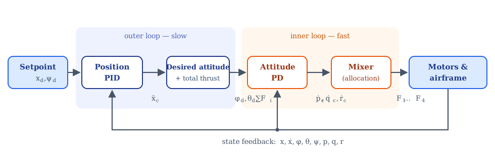
The controller is arranged as a cascade because the vehicle is underactuated. The split holds only while the attitude loop settles much faster than the position loop, which lets the outer loop treat its commanded tilt as achieved immediately. That separation is a requirement you impose when choosing the gains, not something the airframe gives you. Outer loop (slow). A position PID converts position error into a commanded acceleration \(\ddot{\mathbf{x}}_c\) (step 11). Attitude and thrust extraction. \(\ddot{\mathbf{x}}_c\) is converted into a desired tilt \((\phi_d, \theta_d)\) and a total thrust \(\sum F_i\) (steps 12 and 13). Yaw \(\psi_d\) is free and commanded independently. Inner loop (fast). An attitude PD converts attitude error into commanded angular accelerations \((\dot p_c, \dot q_c, \dot r_c)\) (step 14). Allocation. The mixer converts \(\left(\sum F_i, \dot p_c, \dot q_c, \dot r_c\right)\) into four individual rotor thrusts, and then into motor speeds (steps 17 to 21). This is the only part of the controller that knows which airframe it is flying.
Step 11 · Outer loop: position PID shared
We want the position error \(\mathbf{e} = \mathbf{x}_d - \mathbf{x}\) to obey a stable second-order ODE. Imposing \[\left(\ddot{\mathbf{x}}_{d} - \ddot{\mathbf{x}}_{c}\right) + K_d \left(\dot{\mathbf{x}}_{d} - \dot{\mathbf{x}}\right) + K_p \left(\mathbf{x}_d - \mathbf{x}\right) + K_i \int \left(\mathbf{x}_d - \mathbf{x}\right) dt = \mathbf{0} \tag{20}\] and solving for the commanded acceleration gives \[\ddot{\mathbf{x}}_{c} = \ddot{\mathbf{x}}_{d} + K_d \left(\dot{\mathbf{x}}_{d} - \dot{\mathbf{x}}\right) + K_p \left(\mathbf{x}_d - \mathbf{x}\right) + K_i \int \left(\mathbf{x}_d - \mathbf{x}\right) dt \tag{21}\] with diagonal gains \(K_p = \mathrm{diag}(k_{p_x}, k_{p_y}, k_{p_z})\), and likewise \(K_d\), \(K_i\). For station keeping the feedforward term vanishes (\(\ddot{\mathbf{x}}_d = \mathbf{0}\)) and \((21)\) collapses to a plain PID. For trajectory tracking you keep \(\ddot{\mathbf{x}}_d\) and \(\dot{\mathbf{x}}_d\) as feedforward, which lets the vehicle follow a path instead of lagging permanently behind it. Componentwise: \[\ddot{\mathbf{x}}_{c} = \left[\begin{matrix} k_{d_x} (\dot x_{d} - \dot x) + k_{p_x} (x_d - x) + k_{i_x} \int (x_d - x)\, dt \\ k_{d_y} (\dot y_{d} - \dot y) + k_{p_y} (y_d - y) + k_{i_y} \int (y_d - y)\, dt \\ k_{d_z} (\dot z_{d} - \dot z) + k_{p_z} (z_d - z) + k_{i_z} \int (z_d - z)\, dt \end{matrix}\right] = \begin{pmatrix} \ddot x_c \\ \ddot y_c \\ \ddot z_c \end{pmatrix} \tag{22}\] The \(z\) integrator matters here. Neither \(m\) nor \(k_f\) is known exactly, and without the integral term the vehicle settles a little below its altitude setpoint and stays there.
Step 12 · From acceleration to attitude shared
Now invert the translational dynamics. Setting \(\ddot x = \ddot x_c\) and \(\ddot y = \ddot y_c\) in \((14)\) and \((15)\): \[\begin{align} s_\phi s_\psi + s_\theta c_\phi c_\psi &= \frac{m\, \ddot x_c}{\sum_i F_i} \tag{23}\\ -s_\phi c_\psi + s_\psi s_\theta c_\phi &= \frac{m\, \ddot y_c}{\sum_i F_i} \tag{24} \end{align}\] Near hover the tilt angles are small, and the total thrust nearly balances weight: \(\phi \to 0\), so \(\sin\phi \approx \phi\) and \(\cos\phi \approx 1\) \(\theta \to 0\), so \(\sin\theta \approx \theta\) and \(\cos\theta \approx 1\) the rotors very nearly carry the weight, so \(\sum_i F_i \approx mg\) Yaw is not linearized. \(\psi\) can be anything; a hovering vehicle is free to point wherever it likes, so only \(\phi\) and \(\theta\) are assumed small. Keeping \(\sin\psi\) and \(\cos\psi\) exact is what makes the result below work at any heading. If you assume \(\psi \to 0\) as well, \((26)\) holds only at zero heading; at any other heading the commanded tilt comes out rotated by \(\psi\) in the horizontal plane, and the vehicle accelerates at an angle to the direction asked for. With that, \((23)\) and \((24)\) become linear in \(\phi, \theta\): \[\left[\begin{matrix} s_\psi & c_\psi \\ -c_\psi & s_\psi \end{matrix}\right] \begin{pmatrix} \phi \\ \theta \end{pmatrix} = \frac{1}{g} \begin{pmatrix} \ddot x_c \\ \ddot y_c \end{pmatrix} \tag{25}\] That \(2\times2\) matrix has determinant \(s_\psi^2 + c_\psi^2 = 1\), so it is orthogonal and inverts by transposition. There is no singularity here: \[\begin{pmatrix} \phi_{d} \\ \theta_{d} \end{pmatrix} = \frac{1}{g} \left[\begin{matrix} s_\psi & -c_\psi \\ c_\psi & s_\psi \end{matrix}\right] \begin{pmatrix} \ddot x_c \\ \ddot y_c \end{pmatrix} = \frac{1}{g} \begin{pmatrix} \ddot x_c \sin\psi - \ddot y_c \cos\psi \\ \ddot x_c \cos\psi + \ddot y_c \sin\psi \end{pmatrix} \tag{26}\] Sanity check at \(\psi = 0\): \(\theta_d = \ddot x_c / g\) and \(\phi_d = -\ddot y_c / g\). Pitching about \(+y\) tilts the body \(z\)-axis toward \(+x\), so positive pitch buys positive \(x\)-acceleration; rolling about \(+x\) tilts it toward \(-y\), hence the minus sign. Both agree with \((3)\). In practice, make two changes to this. Replace \(g\) with the commanded specific thrust \(\ddot z_c + g\), which is exact rather than a hover approximation, and whose difference from \(g\) grows with the commanded climb rate: \[\phi_d = \frac{\ddot x_c \sin\psi - \ddot y_c \cos\psi}{\ddot z_c + g}, \qquad \theta_d = \frac{\ddot x_c \cos\psi + \ddot y_c \sin\psi}{\ddot z_c + g} \tag{27}\] Then saturate \(\phi_d\) and \(\theta_d\) at some maximum tilt. Where you put that limit is a design choice, traded against how much horizontal acceleration you are willing to give up. The small-angle inversion is the first thing to break when the controller is pushed hard, and without a clamp a large position error can command a flip.
Step 13 · Total thrust shared
From \((16)\), with \(c_\phi c_\theta \approx 1\) near hover: \[\sum_{i=1}^{4} F_{i} = m\left(\ddot z_c + g\right) \tag{28}\] For larger tilts, divide by \(c_\phi c_\theta\) instead, since a banked vehicle needs more thrust to hold altitude. This is usually called tilt compensation, and it writes \((28)\) as \(\sum F_i = m(\ddot z_c + g)/(c_\phi c_\theta)\).
Step 14 · Inner loop: attitude PD shared
The attitude loop drives the body toward \((\phi_d, \theta_d, \psi_d)\) by commanding angular accelerations: \[\begin{pmatrix} \dot p_c \\ \dot q_c \\ \dot r_c \end{pmatrix} = K_{p}^{att} \begin{pmatrix} \phi_{d}-\phi \\ \theta_{d} - \theta \\ \psi_{d} - \psi \end{pmatrix} + K_{d}^{att} \begin{pmatrix} p_{d}-p \\ q_{d} - q \\ r_{d} - r \end{pmatrix} \tag{29}\] with \(K_p^{att}\) and \(K_d^{att}\) diagonal. Equation \((29)\) pairs Euler-angle errors with body-rate errors. That is only legitimate because \(W \approx I\) near hover, where \(p \approx \dot\phi\), \(q \approx \dot\theta\) and \(r \approx \dot\psi\), so \((29)\) really is a PD law on each angle. At large tilt the pairing loses its meaning, and you then have to map the desired Euler rates through \(W\) from \((4)\), or drop Euler angles and use a geometric \(SO(3)\) controller. Also wrap \(\psi_d - \psi\) to \((-\pi, \pi]\). If you forget, a yaw setpoint that crosses \(\pm\pi\) will send the vehicle spinning the long way round.
Step 15 · Simplifying the rotational dynamics shared
To turn \((\dot p_c, \dot q_c, \dot r_c)\) into torques, we use \((17)\) to \((19)\). Near hover two things hold: The yaw rate is small, \(r \approx 0\). The airframe is symmetric about the body \(x\) and \(y\) axes, \(i_{xx} \approx i_{yy}\). The first removes the \(qr\) and \(pr\) terms in \((17)\) and \((18)\), the second removes the \(pq\) term in \((19)\). The gyroscopic coupling drops out, and three decoupled axes are left: \[\tau_x \approx i_{xx}\,\dot p_c, \qquad \tau_y \approx i_{yy}\,\dot q_c, \qquad \tau_z \approx i_{zz}\,\dot r_c \tag{30}\] The second assumption is worth a word for each layout. On a + frame with four equal arms, \(i_{xx} = i_{yy}\) follows from the mass distribution being symmetric under a 90-degree rotation. On an X frame the same symmetry holds, since rotating the rotor set by 90 degrees maps it onto itself in both cases. So the assumption is about the mass being laid out symmetrically, not about which layout was chosen. If you need the model to hold at high yaw rates, keep the full \((17)\) to \((19)\) and add the gyroscopic terms back as feedforward. They are known exactly from the measured \(p, q, r\).
Step 16 · The four demands shared
Both layouts carry the factor \(l\) outside the bracket in their roll and pitch torques, \((9^{+})\) and \((10^{+})\) for +, \((9^{\times})\) and \((10^{\times})\) for X. Dividing those torques by \(l\), and the yaw torque \((7)\) by \(k_m/k_f\), leaves four demands whose units are thrust, and whose definition is the same for both airframes: \[\mathbf{u} = \begin{pmatrix} u_1 \\ u_2 \\ u_3 \\ u_4 \end{pmatrix} = \begin{pmatrix} \textstyle\sum_i F_i \\[2pt] \tau_x / l \\[2pt] \tau_y / l \\[2pt] \tau_z\, k_f / k_m \end{pmatrix} = \left[\begin{matrix} m\left(\ddot z_c + g\right) \\[2pt] \dfrac{i_{xx}\, \dot p_c}{l} \\[6pt] \dfrac{i_{yy}\, \dot q_c}{l} \\[6pt] \dfrac{k_{f}\, i_{zz}\, \dot r_c}{k_{m}} \end{matrix}\right] \tag{31}\] using \((28)\) for the first row and \((30)\) for the other three. Everything to this point has been shared. The remaining question is which combination of \(F_1 \ldots F_4\) delivers a given \(\mathbf{u}\), and that is where the geometry of step 1 finally decides the answer.
Step 17 · The mixer matrix layouts differ
Read the four rows off \((28)\), \((9^{+})\), \((10^{+})\) and \((7)\) in that order. Each row is the coefficient pattern of one demand in terms of \(F_1 \ldots F_4\): \[\underbrace{\left[\begin{matrix} 1 & 1 & 1 & 1 \\ 0 & 1 & 0 & -1 \\ -1 & 0 & 1 & 0 \\ 1 & -1 & 1 & -1 \end{matrix}\right]}_{\mathcal{M}_{+}} \begin{pmatrix} F_{1}\\ F_{2} \\ F_{3}\\ F_{4} \end{pmatrix} = \mathbf{u} \tag{$32^{+}$}\] The zeros in rows 2 and 3 are the actuator decoupling noted in step 7: rotors 1 and 3 do not appear in the roll row, and rotors 2 and 4 do not appear in the pitch row. Its determinant is \(-8\), so the matrix is invertible and the allocation is unique.	Read the four rows off \((28)\), \((9^{\times})\), \((10^{\times})\) and \((7)\) in the same order. The thrust row and the yaw row are unchanged, because neither depended on rotor position; the roll and pitch rows are the ones that move: \[\underbrace{\left[\begin{matrix} 1 & 1 & 1 & 1 \\ 1 & -1 & -1 & 1 \\ -1 & -1 & 1 & 1 \\ 1 & -1 & 1 & -1 \end{matrix}\right]}_{\mathcal{M}_{X}} \begin{pmatrix} F_{1}\\ F_{2} \\ F_{3}\\ F_{4} \end{pmatrix} = \mathbf{u} \tag{$32^{\times}$}\] Every entry is \(\pm 1\); no rotor is absent from any row. Its determinant is \(16\), so the allocation is again unique.
Step 18 · Inverting the mixer layouts differ
Rows 1 and 4 of \((32^{+})\) combine to separate the two diagonal pairs: \[u_1 + u_4 = 2\left(F_1 + F_3\right), \qquad u_1 - u_4 = 2\left(F_2 + F_4\right) \tag{$33^{+}$}\] Row 3 gives the difference within the first pair, \(F_3 - F_1 = u_3\), and row 2 the difference within the second, \(F_2 - F_4 = u_2\). Solving the two sum-and-difference pairs: \[\begin{align} F_1 &= \tfrac{1}{4}(u_1 + u_4) - \tfrac{1}{2}u_3, &\qquad F_3 &= \tfrac{1}{4}(u_1 + u_4) + \tfrac{1}{2}u_3 \notag \\ F_2 &= \tfrac{1}{4}(u_1 - u_4) + \tfrac{1}{2}u_2, &\qquad F_4 &= \tfrac{1}{4}(u_1 - u_4) - \tfrac{1}{2}u_2 \notag \end{align}\] which is exactly \[\mathcal{M}_{+}^{-1} = \left[\begin{matrix} \tfrac{1}{4} & 0 & -\tfrac{1}{2} & \tfrac{1}{4}\\ \tfrac{1}{4} & \tfrac{1}{2} & 0 & -\tfrac{1}{4}\\ \tfrac{1}{4} & 0 & \tfrac{1}{2} & \tfrac{1}{4}\\ \tfrac{1}{4} & -\tfrac{1}{2}& 0 & -\tfrac{1}{4} \end{matrix}\right] \tag{$34^{+}$}\] The weights are \(\tfrac14\) for thrust and yaw, \(\tfrac12\) for roll and pitch, and zero wherever a rotor sits on the axis it cannot torque about.	The four rows of \(\mathcal{M}_{X}\) are mutually orthogonal and each has norm \(2\), so no elimination is needed: \[\mathcal{M}_{X}\,\mathcal{M}_{X}^{T} = 4 I \qquad \Longrightarrow \qquad \mathcal{M}_{X}^{-1} = \tfrac{1}{4}\,\mathcal{M}_{X}^{T} \tag{$33^{\times}$}\] The matrix is \(2\) times an orthogonal matrix, of the \(\pm 1\) Hadamard type. Transposing and scaling: \[\mathcal{M}_{X}^{-1} = \frac{1}{4}\left[\begin{matrix} 1 & 1 & -1 & 1\\ 1 & -1 & -1 & -1\\ 1 & -1 & 1 & 1\\ 1 & 1 & 1 & -1 \end{matrix}\right] \tag{$34^{\times}$}\] Every weight is \(\tfrac14\) and no entry is zero, which is the row orthogonality of \((32^{\times})\) showing up in the inverse.
Step 19 · The rotor thrusts layouts differ
Substituting the demands \((31)\) into \((34^{+})\): \[\begin{pmatrix} F_{1}\\ F_{2} \\ F_{3}\\ F_{4} \end{pmatrix} = \left[\begin{matrix} \frac{m(\ddot z_c + g)}{4} - \frac{i_{yy} \dot q_c}{2l} + \frac{k_{f} i_{zz} \dot r_c}{4 k_{m}} \\[4pt] \frac{m(\ddot z_c + g)}{4} + \frac{i_{xx} \dot p_c}{2l} - \frac{k_{f} i_{zz} \dot r_c}{4 k_{m}} \\[4pt] \frac{m(\ddot z_c + g)}{4} + \frac{i_{yy} \dot q_c}{2l} + \frac{k_{f} i_{zz} \dot r_c}{4 k_{m}} \\[4pt] \frac{m(\ddot z_c + g)}{4} - \frac{i_{xx} \dot p_c}{2l} - \frac{k_{f} i_{zz} \dot r_c}{4 k_{m}} \end{matrix}\right] \tag{$35^{+}$}\] Sign check. A positive roll command \(\dot p_c > 0\) rotates \(+y_b\) toward \(+z_b\), so the rotor on \(+y_b\) must push harder. That is rotor 2, and it is the only one whose thrust rises with \(\dot p_c\). A positive pitch command \(\dot q_c > 0\) needs the rear rotor to push harder, and rotor 3 at \(x = -l\) is the one that does.	Substituting the demands \((31)\) into \((34^{\times})\), and factoring the column so the four channels line up: \[\begin{pmatrix} F_{1}\\ F_{2} \\ F_{3}\\ F_{4} \end{pmatrix} = \left[\begin{matrix} \frac{m}{4} & \frac{i_{xx}}{4l} & -\frac{i_{yy}}{4l} & \frac{k_{f} i_{zz}}{4 k_{m}} \\[4pt] \frac{m}{4} & -\frac{i_{xx}}{4l} & -\frac{i_{yy}}{4l} & -\frac{k_{f} i_{zz}}{4 k_{m}}\\[4pt] \frac{m}{4} & -\frac{i_{xx}}{4l} & \frac{i_{yy}}{4l} & \frac{k_{f} i_{zz}}{4 k_{m}}\\[4pt] \frac{m}{4} & \frac{i_{xx}}{4l} & \frac{i_{yy}}{4l} & -\frac{k_{f} i_{zz}}{4 k_{m}} \end{matrix}\right] \begin{pmatrix} \ddot z_c + g \\ \dot p_c \\ \dot q_c \\ \dot r_c \end{pmatrix} \tag{$35^{\times}$}\] Sign check. A positive roll command \(\dot p_c > 0\) raises the two rotors on \(+y_b\), which are 1 and 4, and lowers 2 and 3. A positive pitch command raises the rear pair 3 and 4 and lowers the front pair 1 and 2. Both patterns match the columns above.
Step 20 · How control effort is spread layouts differ
Take a pure roll demand, \(u_2 \neq 0\) with \(u_1 = u_3 = u_4 = 0\). From column 2 of \((34^{+})\): \[\Delta F_1 = \Delta F_3 = 0, \qquad \Delta F_2 = +\frac{u_2}{2}, \qquad \Delta F_4 = -\frac{u_2}{2} \tag{$36^{+}$}\] Two motors do all the work, at weight \(\tfrac12\) each.	Take the same pure roll demand. From column 2 of \((34^{\times})\): \[\Delta F_1 = \Delta F_4 = +\frac{u_2}{4}, \qquad \Delta F_2 = \Delta F_3 = -\frac{u_2}{4} \tag{$36^{\times}$}\] Four motors share the work, at weight \(\tfrac14\) each.
Put both on the same physical footing. To deliver a roll torque \(\tau_x\) on a frame with center-to-rotor distance \(L\), the + layout has \(l = L\), so it needs \(u_2 = \tau_x / L\) and moves each of two motors by \(\tau_x / (2L)\). The X layout has \(l = L/\sqrt{2}\), so it needs \(u_2 = \sqrt{2}\,\tau_x / L\) and moves each of four motors by \(\tau_x / (2\sqrt{2}\,L)\). The per-motor deviation is smaller by \(1/\sqrt{2} \approx 0.71\), which is step 8 read from the actuator side rather than the torque side. Both mixers are constant matrices, so either one costs four multiply-accumulates per rotor and runs comfortably at the inner-loop rate.
Step 21 · From thrusts to motor commands shared
Finally, invert \((6)\): \[\omega_i = \sqrt{\frac{F_i}{k_f}} \tag{37}\] Clip \(F_i\) at both ends before taking the square root: Clip to \(F_i \ge 0\). A fixed-pitch rotor cannot produce negative thrust, but \((35^{+})\) and \((35^{\times})\) will both ask for it during an aggressive maneuver. Clip to \(F_i \le F_{max}\). Saturating each motor independently rotates the resulting torque vector away from the commanded direction, so the vehicle still flies and the symptom is a sluggish or cross-coupled response rather than an outright failure. Which rotor hits a limit first, and what the vehicle does about it, is the last place the two layouts differ.
Step 22 · What saturation does layouts differ
Roll lives on rotors 2 and 4 alone, so those two clip first. A demand large enough to drive \(F_4\) to zero leaves rotors 1 and 3 with headroom the mixer has no way to spend on roll, because their roll weight in \((34^{+})\) is zero. Clipping \(F_4\) at zero also raises \(\sum_i F_i\) above the value \((28)\) asked for, so the vehicle climbs while under-rolling. Pitch behaves the same way on rotors 1 and 3.	Every channel is spread over all four rotors at weight \(\tfrac14\), so no single channel drives a motor to its limit on its own. From \((35^{\times})\), rotor 1 clips only when \(u_1 + u_2 - u_3 + u_4\) leaves the feasible band, which needs roll, pitch and yaw to line up in sign on that corner. What saturates first is therefore a combined maneuver rather than a pure roll or a pure pitch, and when it does, all four rotors are already near their limits.
The remedy is the same for both airframes: rank the channels, and give the available thrust to them in order. Roll and pitch come first because they keep the vehicle upright, then yaw, and total thrust absorbs whatever is left.

Limitations

This is the standard model, and it holds up well for hover and gentle flight on either airframe. It also leaves out a fair amount, and the omissions are the same for both layouts:

• Rotor gyroscopic torque. The rotors carry angular momentum of their own, so a body rotation produces \(-J_r \Omega_r\,\boldsymbol\omega \times \hat z_b\), where \(J_r\) is the rotor polar inertia and \(\Omega_r\) is the net rotor spin resolved along \(+z_b\). Under the convention used here, rotors 1 and 3 turn in the \(-z_b\) sense and rotors 2 and 4 in the \(+z_b\) sense, so \(\Omega_r = -\omega_1 + \omega_2 - \omega_3 + \omega_4\). Much of the literature writes this with the signs reversed, which corresponds to the opposite spin assignment; note that \(\Omega_r\) is opposite in sign to the yaw-torque pattern in \((7)\), since the reaction torque opposes the spin. The term scales with body rate, so it is small at hover and matters mainly during fast rolls.
• Motor dynamics. \(\omega_i\) is treated as something you can set instantly. A real ESC and motor have a finite rise time, and that time constant puts a ceiling on inner-loop bandwidth.
• Aerodynamics: body drag, blade flapping, induced velocity, ground effect. Blade flapping produces a velocity-dependent pitching moment for which the model above has no term at all, so I would expect it to be the omission that matters first as airspeed rises.
• Off-diagonal inertia, that is, the assumption that the body axes are the principal axes.
• Frame flex. Vibration from the arms couples into the gyros, and is usually filtered rather than modeled.
• Battery sag, which drifts \(k_f\) as the voltage drops. The altitude integrator absorbs most of this.

Summary

Everything from the rigid-body model through to the attitude loop is common to the two airframes:

Quantity	Result
Body \(z\)-axis in world frame, eq. \((3)\)	\((s_\phi s_\psi + s_\theta c_\phi c_\psi,\; -s_\phi c_\psi + s_\psi s_\theta c_\phi,\; c_\phi c_\theta)\)
Translation, eq. \((12)\)	\(m\ddot{\mathbf{x}} = -mg\hat{z}_w + R^{w}_{b}(0,0,\textstyle\sum F_i)^T\)
Rotation, eq. \((13)\)	\(I\dot{\boldsymbol\omega} = \boldsymbol\tau - \boldsymbol\omega \times I\boldsymbol\omega\)
Desired tilt, eq. \((27)\)	\(\phi_d = \frac{\ddot x_c s_\psi - \ddot y_c c_\psi}{\ddot z_c + g}\), \(\;\theta_d = \frac{\ddot x_c c_\psi + \ddot y_c s_\psi}{\ddot z_c + g}\)
Total thrust, eq. \((28)\)	\(\sum F_i = m(\ddot z_c + g)\)
Four demands, eq. \((31)\)	\(\mathbf{u} = (\textstyle\sum F_i,\; \tau_x/l,\; \tau_y/l,\; \tau_z k_f/k_m)^T\)
Yaw torque, eq. \((7)\)	\(\tau_z = \frac{k_m}{k_f}(F_1 - F_2 + F_3 - F_4)\)
Motor command, eq. \((37)\)	\(\omega_i = \sqrt{F_i / k_f}\), after clipping \(F_i\) to \([0, F_{max}]\)

The geometry and the allocation are where they part:

Quantity	+ configuration	X configuration
Rotor positions \((x_i, y_i)\)	\((l,0), (0,l), (-l,0), (0,-l)\)	\((l,l), (l,-l), (-l,-l), (-l,l)\)
Meaning of \(l\)	arm length, \(L = l\)	half-span, \(L = l\sqrt{2}\)
Roll torque	\(\tau_x = l(F_2 - F_4)\)	\(\tau_x = l(F_1 - F_2 - F_3 + F_4)\)
Pitch torque	\(\tau_y = l(-F_1 + F_3)\)	\(\tau_y = l(-F_1 - F_2 + F_3 + F_4)\)
Mixer rows	\((1,1,1,1)\), \((0,1,0,-1)\), \((-1,0,1,0)\), \((1,-1,1,-1)\)	\((1,1,1,1)\), \((1,-1,-1,1)\), \((-1,-1,1,1)\), \((1,-1,1,-1)\)
Determinant	\(-8\)	\(16\)
Inverse	\(\mathcal{M}_{+}^{-1}\), eq. \((34^{+})\)	\(\mathcal{M}_X^{-1} = \tfrac{1}{4}\mathcal{M}_X^{T}\), eq. \((34^{\times})\)
Roll and pitch weights in the inverse	\(\tfrac{1}{2}\) on two rotors, \(0\) on the other two	\(\tfrac{1}{4}\) on all four
Roll torque at equal \(L\), per \(\Delta F\)	\(2L\,\Delta F\)	\(2\sqrt{2}\,L\,\Delta F\)

Thrust acts only along \(+z_b\) on either airframe, so horizontal motion requires tilt. The outer loop chooses a direction for \(\hat z_b\), the inner loop drives the airframe to the attitude that achieves it, and the mixer distributes the four resulting demands over four rotors subject to \(F_i \ge 0\). The + layout spends that budget on two motors per axis and the X layout on four, which is the whole of the difference between them.

Note

If you come across any errors, please let me know. I will be happy to fix it.
Happy reading!!

References

1. R. Mahony, V. Kumar and P. Corke, “Multirotor Aerial Vehicles: Modeling, Estimation, and Control of Quadrotor,” IEEE Robotics & Automation Magazine, vol. 19, no. 3, pp. 20–32, 2012.
2. D. Mellinger and V. Kumar, “Minimum snap trajectory generation and control for quadrotors,” IEEE ICRA, 2011.
3. T. Lee, M. Leok and N. H. McClamroch, “Geometric tracking control of a quadrotor UAV on SE(3),” IEEE CDC, 2010.
4. F. Hover and M. Triantafyllou, “System Design for Uncertainty,” MIT OCW 2.017J, chapter on rotations.